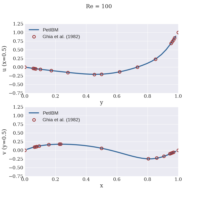
2D lid-driven cavity flow at Re=100
Input files are located in the folder examples/navierstokes/liddrivencavity2dRe100 of the PetIBM directory.
If PetIBM is not installed using conda/mamba, make sure that the PetIBM executables are available in your PATH environment variable. To add the PetIBM installation directory to you PATH:
export PATH=<petibm-installation-directory>:$PATH
We are going to solve the flow in a 2D square cavity of unit length with the top wall moving in the positive x direction at speed 1. The Reynolds number (based on the kinematic viscosity, the length of the cavity, and the speed of the moving wall) is 100. The fluid is initially at rest and the top wall impulsively starts moving.
The computational domain [0, 1]x[0, 1] is uniformly discretized with 32 cells in each direction.
We will run 1000 time steps with a time increment of 0.01 and save the numerical solution at the end.
To run this example:
cd <simulation-directory>
petibm-navierstokes
The simulation should completes within few seconds.
The numerical solution is saved in the sub-folder solution.
We provide a Python script to visualize the velocity components along the centerlines and compare with the numerical results from Ghia et al. (1982). To run the script:
python scripts/plotCenterlineVelocities.py
The plot will be saved as a PNG file in the folder figures of the simulation directory.
Here is what we obtained:
You can also run the utility petibm-vorticity to compute and write the 2D vorticity field at saved time steps:
petibm-vorticity
The field wz will be written in the time-step HDF5 files; the grid for the vorticity is also written in the file grid.h5 under the group wz.
Next, you can create XDMF files for the field variables with the utility
petibm-createxdmf
It will create XDMF files for the pressure (p.xmf), the velocity components (u.xmf and v.xmf), and the vorticity (wz.xmf). These files can be open with VisIt to read, visualize, and process the field solutions.
2D flow over a circular cylinder at Re=40
Input files are located in the folder examples/ibpm/cylinder2dRe40 of the PetIBM directory.
If PetIBM is not installed using conda/mamba, make sure that the PetIBM executables are available in your PATH environment variable. To add the PetIBM installation directory to you PATH:
export PATH=<petibm-installation-directory>:$PATH
A circular cylinder of diameter 1.0 is placed at the center of a two-dimensional domain spanning [-15,15]x[-15,15]. The initial velocity of the fluid in the domain is (1, 0). Dirichlet conditions for the velocity are set on all boundaries (velocity set to (1, 0)), except at the outlet where the fluid is convected outside the domain in the x-direction at speed 1.0. The Reynolds number (based on the freestream speed, the diameter of the circular cylinder, and the kinematic viscosity) is 40.
The computational domain is discretized using an stretched Cartesian grid with 186x186 cells. The mesh is kept uniform in the sub-domain [-0.6, 0.6]x[-0.6, 0.6] and stretched to the external boundaries with a constant ratio of 1.05.
For this example, we will run the simulation with the immersed-boundary projection method (Taira and Colonius, 2007) for 2000 time steps with a time increment of 0.01 and save the numerical solution at the end.
To run the example using 2 MPI processes:
cd <simulation-directory>
mpiexec -np 2 petibm-ibpm
The run should complete in less than 5 minutes and the numerical solution is saved in the folder solution.
We provide a Python script (located under the folder scripts in the simulation directory) to plot the instantaneous drag coefficient and compare it with the numerical results from Koumoutsakos and Leonard (1995). To run the script:
python scripts/plotDragCoefficient.py
You can also run the utility petibm-vorticity to compute and write the 2D vorticity field at saved time steps:
petibm-vorticity
The field wz will be written in the time-step HDF5 files; the grid for the vorticity is also written in the file grid.h5 under the group wz.
We also provide a Python script to plot the vorticity field and save it in the folder figures in the simulation directory:
python scripts/plotVorticity.py
Here is what we obtained:


Next, you can create XDMF files for the field variables with the utility
petibm-createxdmf
It will create XDMF files for the pressure (p.xmf), the velocity components (u.xmf and v.xmf), and the vorticity (wz.xmf). These files can be open with VisIt to read, visualize, and process the field solutions.
2D flow over a circular cylinder at Re=550 (using AmgX)
Input files are located in the folder examples/ibpm/cylinder2dRe550_GPU of the PetIBM directory.
If PetIBM is not installed using conda/mamba, make sure that the PetIBM executables are available in your PATH environment variable. To add the PetIBM installation directory to you PATH:
export PATH=<petibm-installation-directory>:$PATH
A circular cylinder of diameter 1.0 is placed at the center of a two-dimensional domain spanning [-15,15]x[-15,15]. The initial velocity of the fluid in the domain is (1, 0). Dirichlet conditions for the velocity are set on all boundaries (velocity set to (1, 0)), except at the outlet where the fluid is convected outside the domain in the x-direction at speed 1.0. The Reynolds number (based on the freestream speed, the diameter of the circular cylinder, and the kinematic viscosity) is 550.
The computational domain is discretized using an stretched Cartesian grid with 450x450 cells. The mesh is kept uniform in the sub-domain [-0.54, 0.54]x[-0.54, 0.54] and stretched to the external boundaries with a constant ratio of 1.02.
For this example, we will run the simulation with the immersed-boundary projection method (Taira and Colonius, 2007) for 1200 time steps with a time increment of 0.0025 and save the numerical solution at the end.
To run the example using 2 MPI processes and 1 CUDA-capable GPU device:
cd <simulation-directory>
export CUDA_VISIBLE_DEVICES=0
mpiexec -np 2 petibm-ibpm
The run should complete in less than 5 minutes (with a NVIDIA K40 GPU device) and the numerical solution is saved in the folder solution. The MPI flag --mca opal_cuda_support 1 may be needed if using Anaconda's OpenMPI package.
We provide a Python script (located under the folder scripts in the simulation directory) to plot the instantaneous drag coefficient and compare it with the numerical results from Koumoutsakos and Leonard (1995). To run the script:
python scripts/plotDragCoefficient.py
You can also run the utility petibm-vorticity to compute and write the 2D vorticity field at saved time steps:
petibm-vorticity
The field wz will be written in the time-step HDF5 files; the grid for the vorticity is also written in the file grid.h5 under the group wz.
We also provide a Python script to plot the vorticity field and save it in the folder figures in the simulation directory:
python scripts/plotVorticity.py
Here is what we obtained:


Next, you can create XDMF files for the field variables with the utility
petibm-createxdmf
It will create XDMF files for the pressure (p.xmf), the velocity components (u.xmf and v.xmf), and the vorticity (wz.xmf). These files can be open with VisIt to read, visualize, and process the field solutions.
References
- Ghia, U. K. N. G., Ghia, K. N., & Shin, C. T. (1982). High-Re solutions for incompressible flow using the Navier-Stokes equations and a multigrid method. Journal of computational physics, 48(3), 387-411.
- Koumoutsakos, P., & Leonard, A. (1995). High-resolution simulations of the flow around an impulsively started cylinder using vortex methods. Journal of Fluid Mechanics, 296, 1-38.
- Taira, K., & Colonius, T. (2007). The immersed boundary method: a projection approach. Journal of Computational Physics, 225(2), 2118-2137.