3D examples

3D flow around an inclined flat plate (using NVIDIA AmgX)

The simulations compute the flow past an inclined flat plate, with aspect ratio AR=2, at Reynolds number 100 (based on the chord length of the plate, the freestream velocity, and the kinematic viscosity) in the domain [-4, 6.1]x[-5, 5]x[-5,5]. The fluid velocity is initially set to the freestream velocity. The mesh contains 127x56x84 cells and is uniform in the sub-domain [-0.5, 0.7]x[-0.6, 0.6]x[-1.2, 1.2] with a grid cell-width of 0.04 in the three directions and stretched to the external boundaries with a geometric ratio of 1.03 in the x directions and 1.3 in the y and z directions.

We set freestream conditions for the velocity at the on all boundaries, except at the outlet where we use a convective conditions.

The flat plate has an aspect ratio of 2 ,is centered in the computational domain, and is uniformly discretized with the same resolution than the background Eulerian mesh. In this study, the angle of attack of the plate varies from 0 to 90 degrees with 10-degree increments.

The convective and diffusive terms are temporally integrated with a second-order Adams-Bashforth scheme and a second-order Crank-Nicolson scheme, respectively. Each configuration was run for 2000 time steps with a time-step size of 0.01.

All input files are located in directory examples/decoupledibpm/flatplate3dRe100_GPU:

flatplate3dRe100_GPU:
  ˫ AoA0
  ˫ AoA10
  ˫ AoA20
  ˫ AoA30
  ˫ AoA40
  ˫ AoA50
  ˫ AoA60
  ˫ AoA70
  ˫ AoA80
  ˫ AoA90
  ˫ configs
    ˫ forces_solver.txt
    ˫ poisson_solver.txt
    ˫ velocity_solver.txt
  ˫ README.md
  ˫ scripts
    ˫ plotForceCoefficients.py

The sub-folder configs contains the configuration files for the iterative solvers. In this example, both the Poisson system and the velocity system are solved on GPU with NVIDIA AmgX library.

For this example, we use the decoupled version of the immersed-boundary projection method (Li et al., 2016); executable petibm-decoupledibpm.

When we use 4 MPI processes (Intel(R) Core(TM) i7-3770 CPU @ 3.40GHz) and 1 GPU device (NVIDIA K40), each run finished in less than 8 minutes.

To run the series of simulations:

cd flatplate3dRe100_GPU
# Declare list of angles of attack to run
angles=(0 10 20 30 40 50 60 70 80 90)
for angle in ${angles[@]}; do
    echo "*** Angle of attack: $angle degrees ***"
    # Generate immersed boundary points
    python "AoA$angle/scripts/createBody.py"
    # Run PetIBM
    mpiexec -np 4 petibm-decoupledibpm \
        -directory "AoA$angle" \
        -options_left \
        -log_view ascii:"AoA$angle/stdout.txt"
done

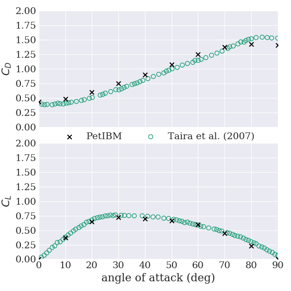
Once all simulations completed, we provide a Python script to plot the force coefficients versus the angle of attack and compare our results with experimental data from Taira et al. (2007). To post-process the force coefficients:

python scripts/plotForceCoefficients.py

The figure will be saved in the sub-folder figures.

Here is what we obtained:

flatplate3dRe100_forceCoefficients

References

• Li, R. Y., Xie, C. M., Huang, W. X., & Xu, C. X. (2016). An efficient immersed boundary projection method for flow over complex/moving boundaries. Computers & Fluids, 140, 122-135.
• Taira, K., Dickson, W. B., Colonius, T., Dickinson, M. H., & Rowley, C. W. (2007). Unsteadiness in flow over a flat plate at angle-of-attack at low Reynolds numbers. AIAA Paper, 710, 2007.